An Introduction to Stock Market Data Analysis with Python (Part 2)

THIS POST IS OUT OF DATE: AN UPDATE OF THIS POST’S INFORMATION IS AT THIS LINK HERE! (Also I bet that WordPress.com just garbled the code in this post.)

I’m keeping this post up for the sake of preserving a record.

This post is the second in a two-part series on stock data analysis using Python, based on a lecture I gave on the subject for MATH 3900 (Data Mining) at the University of Utah (read part 1 here). In these posts, I will discuss basics such as obtaining the data from Yahoo! Finance using pandas, visualizing stock data, moving averages, developing a moving-average crossover strategy, backtesting, and benchmarking. This second post discusses topics including divising a moving average crossover strategy, backtesting, and benchmarking, along with practice problems for readers to ponder.

NOTE: The information in this post is of a general nature containing information and opinions from the author’s perspective. None of the content of this post should be considered financial advice. Furthermore, any code written here is provided without any form of guarantee. Individuals who choose to use it do so at their own risk.

Trading Strategy

Call an open position a trade that will be terminated in the future when a condition is met. A long position is one in which a profit is made if the financial instrument traded increases in value, and a short position is on in which a profit is made if the financial asset being traded decreases in value. When trading stocks directly, all long positions are bullish and all short position are bearish. That said, a bullish attitude need not be accompanied by a long position, and a bearish attitude need not be accompanied by a short position (this is particularly true when trading stock options).

Here is an example. Let’s say you buy a stock with the expectation that the stock will increase in value, with a plan to sell the stock at a higher price. This is a long position: you are holding a financial asset for which you will profit if the asset increases in value. Your potential profit is unlimited, and your potential losses are limited by the price of the stock since stock prices never go below zero. On the other hand, if you expect a stock to decrease in value, you may borrow the stock from a brokerage firm and sell it, with the expectation of buying the stock back later at a lower price, thus earning you a profit. This is called shorting a stock, and is a short position, since you will earn a profit if the stock drops in value. The potential profit from shorting a stock is limited by the price of the stock (the best you can do is have the stock become worth nothing; you buy it back for free), while the losses are unlimited, since you could potentially spend an arbitrarily large amount of money to buy the stock back. Thus, a broker will expect an investor to be in a very good financial position before allowing the investor to short a stock.

Any trader must have a set of rules that determine how much of her money she is willing to bet on any single trade. For example, a trader may decide that under no circumstances will she risk more than 10% of her portfolio on a trade. Additionally, in any trade, a trader must have an exit strategy, a set of conditions determining when she will exit the position, for either profit or loss. A trader may set a target, which is the minimum profit that will induce the trader to leave the position. Likewise, a trader must have a maximum loss she is willing to tolerate; if potential losses go beyond this amount, the trader will exit the position in order to prevent any further loss (this is usually done by setting a stop-loss order, an order that is triggered to prevent further losses).

We will call a plan that includes trading signals for prompting trades, a rule for deciding how much of the portfolio to risk on any particular strategy, and a complete exit strategy for any trade an overall trading strategy. Our concern now is to design and evaluate trading strategies.

We will suppose that the amount of money in the portfolio involved in any particular trade is a fixed proportion; 10% seems like a good number. We will also say that for any trade, if losses exceed 20% of the value of the trade, we will exit the position. Now we need a means for deciding when to enter position and when to exit for a profit.

Here, I will be demonstrating a moving average crossover strategy. We will use two moving averages, one we consider “fast”, and the other “slow”. The strategy is:

• Trade the asset when the fast moving average crosses over the slow moving average.
• Exit the trade when the fast moving average crosses over the slow moving average again.

A long trade will be prompted when the fast moving average crosses from below to above the slow moving average, and the trade will be exited when the fast moving average crosses below the slow moving average later. A short trade will be prompted when the fast moving average crosses below the slow moving average, and the trade will be exited when the fast moving average later crosses above the slow moving average.

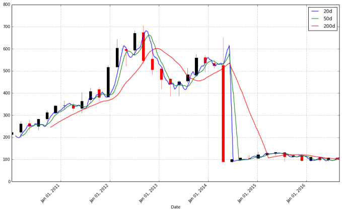
We now have a complete strategy. But before we decide we want to use it, we should try to evaluate the quality of the strategy first. The usual means for doing so is backtesting, which is looking at how profitable the strategy is on historical data. For example, looking at the above chart’s performance on Apple stock, if the 20-day moving average is the fast moving average and the 50-day moving average the slow, this strategy does not appear to be very profitable, at least not if you are always taking long positions.

Let’s see if we can automate the backtesting task. We first identify when the 20-day average is below the 50-day average, and vice versa.

apple['20d-50d'] = apple['20d'] - apple['50d']
apple.tail()

	Open	High	Low	Close	Volume	Adj Close	20d	50d	200d	20d-50d
Date
2016-08-26	107.410004	107.949997	106.309998	106.940002	27766300	106.940002	107.87	101.51	102.73	6.36
2016-08-29	106.620003	107.440002	106.290001	106.820000	24970300	106.820000	107.91	101.74	102.68	6.17
2016-08-30	105.800003	106.500000	105.500000	106.000000	24863900	106.000000	107.98	101.96	102.63	6.02
2016-08-31	105.660004	106.570000	105.639999	106.099998	29662400	106.099998	108.00	102.16	102.60	5.84
2016-09-01	106.139999	106.800003	105.620003	106.730003	26643600	106.730003	108.04	102.39	102.56	5.65

We will refer to the sign of this difference as the regime; that is, if the fast moving average is above the slow moving average, this is a bullish regime (the bulls rule), and a bearish regime (the bears rule) holds when the fast moving average is below the slow moving average. I identify regimes with the following code.

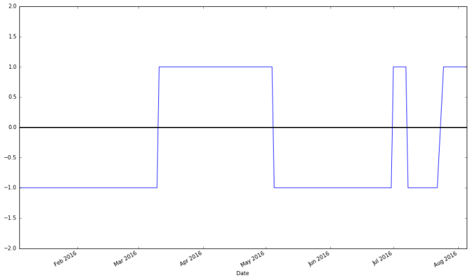
# np.where() is a vectorized if-else function, where a condition is checked for each component of a vector, and the first argument passed is used when the condition holds, and the other passed if it does not
apple["Regime"] = np.where(apple['20d-50d'] > 0, 1, 0)
# We have 1's for bullish regimes and 0's for everything else. Below I replace bearish regimes's values with -1, and to maintain the rest of the vector, the second argument is apple["Regime"]
apple["Regime"] = np.where(apple['20d-50d'] < 0, -1, apple["Regime"])
apple.loc['2016-01-01':'2016-08-07',"Regime"].plot(ylim = (-2,2)).axhline(y = 0, color = "black", lw = 2)

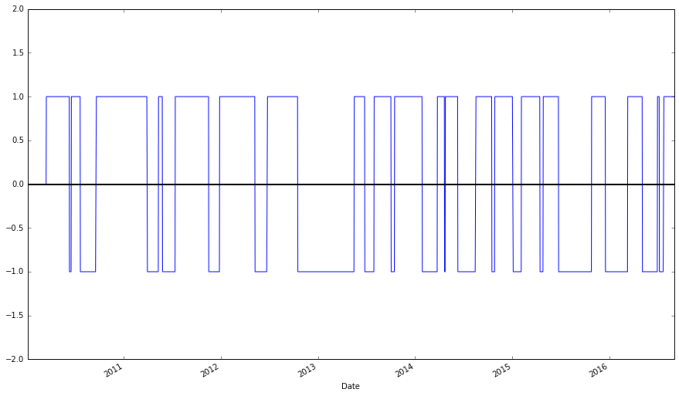
apple["Regime"].plot(ylim = (-2,2)).axhline(y = 0, color = "black", lw = 2)

apple["Regime"].value_counts()

 1    966
-1    663
 0     50
Name: Regime, dtype: int64

The last line above indicates that for 1005 days the market was bearish on Apple, while for 600 days the market was bullish, and it was neutral for 54 days.

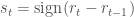
Trading signals appear at regime changes. When a bullish regime begins, a buy signal is triggered, and when it ends, a sell signal is triggered. Likewise, when a bearish regime begins, a sell signal is triggered, and when the regime ends, a buy signal is triggered (this is of interest only if you ever will short the stock, or use some derivative like a stock option to bet against the market).

It’s simple to obtain signals. Let indicate the regime at time , and the signal at time . Then:

, with indicating “sell”, indicating “buy”, and no action. We can obtain signals like so:

# To ensure that all trades close out, I temporarily change the regime of the last row to 0
regime_orig = apple.ix[-1, "Regime"]
apple.ix[-1, "Regime"] = 0
apple["Signal"] = np.sign(apple["Regime"] - apple["Regime"].shift(1))
# Restore original regime data
apple.ix[-1, "Regime"] = regime_orig
apple.tail()

	Open	High	Low	Close	Volume	Adj Close	20d	50d	200d	20d-50d	Regime	Signal
Date
2016-08-26	107.410004	107.949997	106.309998	106.940002	27766300	106.940002	107.87	101.51	102.73	6.36	1.0	0.0
2016-08-29	106.620003	107.440002	106.290001	106.820000	24970300	106.820000	107.91	101.74	102.68	6.17	1.0	0.0
2016-08-30	105.800003	106.500000	105.500000	106.000000	24863900	106.000000	107.98	101.96	102.63	6.02	1.0	0.0
2016-08-31	105.660004	106.570000	105.639999	106.099998	29662400	106.099998	108.00	102.16	102.60	5.84	1.0	0.0
2016-09-01	106.139999	106.800003	105.620003	106.730003	26643600	106.730003	108.04	102.39	102.56	5.65	1.0	-1.0

apple["Signal"].plot(ylim = (-2, 2))

apple["Signal"].value_counts()

 0.0    1637
-1.0      21
 1.0      20
Name: Signal, dtype: int64

We would buy Apple stock 23 times and sell Apple stock 23 times. If we only go long on Apple stock, only 23 trades will be engaged in over the 6-year period, while if we pivot from a long to a short position every time a long position is terminated, we would engage in 23 trades total. (Bear in mind that trading more frequently isn’t necessarily good; trades are never free.)

You may notice that the system as it currently stands isn’t very robust, since even a fleeting moment when the fast moving average is above the slow moving average triggers a trade, resulting in trades that end immediately (which is bad if not simply because realistically every trade is accompanied by a fee that can quickly erode earnings). Additionally, every bullish regime immediately transitions into a bearish regime, and if you were constructing trading systems that allow both bullish and bearish bets, this would lead to the end of one trade immediately triggering a new trade that bets on the market in the opposite direction, which again seems finnicky. A better system would require more evidence that the market is moving in some particular direction. But we will not concern ourselves with these details for now.

Let’s now try to identify what the prices of the stock is at every buy and every sell.

apple.loc[apple["Signal"] == 1, "Close"]

Date
2010-03-16    224.449997
2010-06-18    274.070011
2010-09-20    283.230007
2011-05-12    346.569988
2011-07-14    357.770004
2011-12-28    402.640003
2012-06-25    570.770020
2013-05-17    433.260010
2013-07-31    452.529984
2013-10-16    501.110001
2014-03-26    539.779991
2014-04-25    571.939980
2014-08-18     99.160004
2014-10-28    106.739998
2015-02-05    119.940002
2015-04-28    130.559998
2015-10-27    114.550003
2016-03-11    102.260002
2016-07-01     95.889999
2016-07-25     97.339996
Name: Close, dtype: float64

apple.loc[apple["Signal"] == -1, "Close"]

Date
2010-06-11    253.509995
2010-07-22    259.020000
2011-03-30    348.630009
2011-03-31    348.510006
2011-05-27    337.409992
2011-11-17    377.410000
2012-05-09    569.180023
2012-10-17    644.610001
2013-06-26    398.069992
2013-10-03    483.409996
2014-01-28    506.499977
2014-04-22    531.700020
2014-06-11     93.860001
2014-10-17     97.669998
2015-01-05    106.250000
2015-04-16    126.169998
2015-06-25    127.500000
2015-12-18    106.029999
2016-05-05     93.239998
2016-07-08     96.680000
2016-09-01    106.730003
Name: Close, dtype: float64

# Create a DataFrame with trades, including the price at the trade and the regime under which the trade is made.
apple_signals = pd.concat([
        pd.DataFrame({"Price": apple.loc[apple["Signal"] == 1, "Close"],
                     "Regime": apple.loc[apple["Signal"] == 1, "Regime"],
                     "Signal": "Buy"}),
        pd.DataFrame({"Price": apple.loc[apple["Signal"] == -1, "Close"],
                     "Regime": apple.loc[apple["Signal"] == -1, "Regime"],
                     "Signal": "Sell"}),
    ])
apple_signals.sort_index(inplace = True)
apple_signals

	Price	Regime	Signal
Date
2010-03-16	224.449997	1.0	Buy
2010-06-11	253.509995	-1.0	Sell
2010-06-18	274.070011	1.0	Buy
2010-07-22	259.020000	-1.0	Sell
2010-09-20	283.230007	1.0	Buy
2011-03-30	348.630009	0.0	Sell
2011-03-31	348.510006	-1.0	Sell
2011-05-12	346.569988	1.0	Buy
2011-05-27	337.409992	-1.0	Sell
2011-07-14	357.770004	1.0	Buy
2011-11-17	377.410000	-1.0	Sell
2011-12-28	402.640003	1.0	Buy
2012-05-09	569.180023	-1.0	Sell
2012-06-25	570.770020	1.0	Buy
2012-10-17	644.610001	-1.0	Sell
2013-05-17	433.260010	1.0	Buy
2013-06-26	398.069992	-1.0	Sell
2013-07-31	452.529984	1.0	Buy
2013-10-03	483.409996	-1.0	Sell
2013-10-16	501.110001	1.0	Buy
2014-01-28	506.499977	-1.0	Sell
2014-03-26	539.779991	1.0	Buy
2014-04-22	531.700020	-1.0	Sell
2014-04-25	571.939980	1.0	Buy
2014-06-11	93.860001	-1.0	Sell
2014-08-18	99.160004	1.0	Buy
2014-10-17	97.669998	-1.0	Sell
2014-10-28	106.739998	1.0	Buy
2015-01-05	106.250000	-1.0	Sell
2015-02-05	119.940002	1.0	Buy
2015-04-16	126.169998	-1.0	Sell
2015-04-28	130.559998	1.0	Buy
2015-06-25	127.500000	-1.0	Sell
2015-10-27	114.550003	1.0	Buy
2015-12-18	106.029999	-1.0	Sell
2016-03-11	102.260002	1.0	Buy
2016-05-05	93.239998	-1.0	Sell
2016-07-01	95.889999	1.0	Buy
2016-07-08	96.680000	-1.0	Sell
2016-07-25	97.339996	1.0	Buy
2016-09-01	106.730003	1.0	Sell

# Let's see the profitability of long trades
apple_long_profits = pd.DataFrame({
        "Price": apple_signals.loc[(apple_signals["Signal"] == "Buy") &
                                  apple_signals["Regime"] == 1, "Price"],
        "Profit": pd.Series(apple_signals["Price"] - apple_signals["Price"].shift(1)).loc[
            apple_signals.loc[(apple_signals["Signal"].shift(1) == "Buy") & (apple_signals["Regime"].shift(1) == 1)].index
        ].tolist(),
        "End Date": apple_signals["Price"].loc[
            apple_signals.loc[(apple_signals["Signal"].shift(1) == "Buy") & (apple_signals["Regime"].shift(1) == 1)].index
        ].index
    })
apple_long_profits

	End Date	Price	Profit
Date
2010-03-16	2010-06-11	224.449997	29.059998
2010-06-18	2010-07-22	274.070011	-15.050011
2010-09-20	2011-03-30	283.230007	65.400002
2011-05-12	2011-05-27	346.569988	-9.159996
2011-07-14	2011-11-17	357.770004	19.639996
2011-12-28	2012-05-09	402.640003	166.540020
2012-06-25	2012-10-17	570.770020	73.839981
2013-05-17	2013-06-26	433.260010	-35.190018
2013-07-31	2013-10-03	452.529984	30.880012
2013-10-16	2014-01-28	501.110001	5.389976
2014-03-26	2014-04-22	539.779991	-8.079971
2014-04-25	2014-06-11	571.939980	-478.079979
2014-08-18	2014-10-17	99.160004	-1.490006
2014-10-28	2015-01-05	106.739998	-0.489998
2015-02-05	2015-04-16	119.940002	6.229996
2015-04-28	2015-06-25	130.559998	-3.059998
2015-10-27	2015-12-18	114.550003	-8.520004
2016-03-11	2016-05-05	102.260002	-9.020004
2016-07-01	2016-07-08	95.889999	0.790001
2016-07-25	2016-09-01	97.339996	9.390007

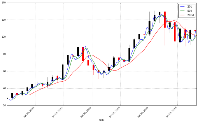
Above, we can see that on May 17th, 2013, there was a massive drop in the price of Apple stock, and it looks like our trading system would do badly. But this price drop is not because of a massive shock to Apple, but simply due to a stock split. And while dividend payments are not as obvious as a stock split, they may be affecting the performance of our system.

# Let's see the result over the whole period for which we have Apple data
pandas_candlestick_ohlc(apple, stick = 45, otherseries = ["20d", "50d", "200d"])

We don’t want our trading system to be behaving poorly because of stock splits and dividend payments. How should we handle this? One approach would be to obtain historical stock split and dividend payment data and design a trading system for handling these. This would most realistically represent the behavior of the stock and could be considered the best solution, but it is more complicated. Another solution would be to adjust the prices to account for stock splits and dividend payments.

Yahoo! Finance only provides the adjusted closing price of a stock, but this is all we need to get adjusted opening, high, and low prices. The adjusted close is computed like so:

where is the multiplier used for the adjustment. Solving for requires only division and thus we can use the closing price and the adjusted closing price to adjust all prices in the series.

Let’s go back, adjust the apple data, and reevaluate our trading system using the adjusted data.

def ohlc_adj(dat):
    """
    :param dat: pandas DataFrame with stock data, including "Open", "High", "Low", "Close", and "Adj Close", with "Adj Close" containing adjusted closing prices

    :return: pandas DataFrame with adjusted stock data

    This function adjusts stock data for splits, dividends, etc., returning a data frame with
    "Open", "High", "Low" and "Close" columns. The input DataFrame is similar to that returned
    by pandas Yahoo! Finance API.
    """
    return pd.DataFrame({"Open": dat["Open"] * dat["Adj Close"] / dat["Close"],
                       "High": dat["High"] * dat["Adj Close"] / dat["Close"],
                       "Low": dat["Low"] * dat["Adj Close"] / dat["Close"],
                       "Close": dat["Adj Close"]})

apple_adj = ohlc_adj(apple)

# This next code repeats all the earlier analysis we did on the adjusted data

apple_adj["20d"] = np.round(apple_adj["Close"].rolling(window = 20, center = False).mean(), 2)
apple_adj["50d"] = np.round(apple_adj["Close"].rolling(window = 50, center = False).mean(), 2)
apple_adj["200d"] = np.round(apple_adj["Close"].rolling(window = 200, center = False).mean(), 2)

apple_adj['20d-50d'] = apple_adj['20d'] - apple_adj['50d']
# np.where() is a vectorized if-else function, where a condition is checked for each component of a vector, and the first argument passed is used when the condition holds, and the other passed if it does not
apple_adj["Regime"] = np.where(apple_adj['20d-50d'] > 0, 1, 0)
# We have 1's for bullish regimes and 0's for everything else. Below I replace bearish regimes's values with -1, and to maintain the rest of the vector, the second argument is apple["Regime"]
apple_adj["Regime"] = np.where(apple_adj['20d-50d'] < 0, -1, apple_adj["Regime"])
# To ensure that all trades close out, I temporarily change the regime of the last row to 0
regime_orig = apple_adj.ix[-1, "Regime"]
apple_adj.ix[-1, "Regime"] = 0
apple_adj["Signal"] = np.sign(apple_adj["Regime"] - apple_adj["Regime"].shift(1))
# Restore original regime data
apple_adj.ix[-1, "Regime"] = regime_orig

# Create a DataFrame with trades, including the price at the trade and the regime under which the trade is made.
apple_adj_signals = pd.concat([
        pd.DataFrame({"Price": apple_adj.loc[apple_adj["Signal"] == 1, "Close"],
                     "Regime": apple_adj.loc[apple_adj["Signal"] == 1, "Regime"],
                     "Signal": "Buy"}),
        pd.DataFrame({"Price": apple_adj.loc[apple_adj["Signal"] == -1, "Close"],
                     "Regime": apple_adj.loc[apple_adj["Signal"] == -1, "Regime"],
                     "Signal": "Sell"}),
    ])
apple_adj_signals.sort_index(inplace = True)
apple_adj_long_profits = pd.DataFrame({
        "Price": apple_adj_signals.loc[(apple_adj_signals["Signal"] == "Buy") &
                                  apple_adj_signals["Regime"] == 1, "Price"],
        "Profit": pd.Series(apple_adj_signals["Price"] - apple_adj_signals["Price"].shift(1)).loc[
            apple_adj_signals.loc[(apple_adj_signals["Signal"].shift(1) == "Buy") & (apple_adj_signals["Regime"].shift(1) == 1)].index
        ].tolist(),
        "End Date": apple_adj_signals["Price"].loc[
            apple_adj_signals.loc[(apple_adj_signals["Signal"].shift(1) == "Buy") & (apple_adj_signals["Regime"].shift(1) == 1)].index
        ].index
    })

pandas_candlestick_ohlc(apple_adj, stick = 45, otherseries = ["20d", "50d", "200d"])

apple_adj_long_profits

	End Date	Price	Profit
Date
2010-03-16	2010-06-10	29.355667	3.408371
2010-06-18	2010-07-22	35.845436	-1.968381
2010-09-20	2011-03-30	37.043466	8.553623
2011-05-12	2011-05-27	45.327660	-1.198030
2011-07-14	2011-11-17	46.792503	2.568702
2011-12-28	2012-05-09	52.661020	21.781659
2012-06-25	2012-10-17	74.650634	10.019459
2013-05-17	2013-06-26	57.882798	-4.701326
2013-07-31	2013-10-04	60.457234	4.500835
2013-10-16	2014-01-28	67.389473	1.122523
2014-03-11	2014-03-17	72.948554	-1.272298
2014-03-24	2014-04-22	73.370393	-1.019203
2014-04-25	2014-10-17	77.826851	16.191371
2014-10-28	2015-01-05	102.749105	-0.028185
2015-02-05	2015-04-16	116.413846	6.046838
2015-04-28	2015-06-26	126.721620	-3.184117
2015-10-27	2015-12-18	112.152083	-7.897288
2016-03-10	2016-05-05	100.015950	-7.278331
2016-06-23	2016-06-27	95.582210	-4.038123
2016-06-30	2016-07-11	95.084904	1.372569
2016-07-25	2016-09-01	96.815526	9.914477

As you can see, adjusting for dividends and stock splits makes a big difference. We will use this data from now on.

Let’s now create a simulated portfolio of $1,000,000, and see how it would behave, according to the rules we have established. This includes:

• Investing only 10% of the portfolio in any trade
• Exiting the position if losses exceed 20% of the value of the trade.

When simulating, bear in mind that:

• Trades are done in batches of 100 stocks.
• Our stop-loss rule involves placing an order to sell the stock the moment the price drops below the specified level. Thus we need to check whether the lows during this period ever go low enough to trigger the stop-loss. Realistically, unless we buy a put option, we cannot guarantee that we will sell the stock at the price we set at the stop-loss, but we will use this as the selling price anyway for the sake of simplicity.
• Every trade is accompanied by a commission to the broker, which should be accounted for. I do not do so here.

Here’s how a backtest may look:

# We need to get the low of the price during each trade.
tradeperiods = pd.DataFrame({"Start": apple_adj_long_profits.index,
                            "End": apple_adj_long_profits["End Date"]})
apple_adj_long_profits["Low"] = tradeperiods.apply(lambda x: min(apple_adj.loc[x["Start"]:x["End"], "Low"]), axis = 1)
apple_adj_long_profits

	End Date	Price	Profit	Low
Date
2010-03-16	2010-06-10	29.355667	3.408371	26.059775
2010-06-18	2010-07-22	35.845436	-1.968381	31.337127
2010-09-20	2011-03-30	37.043466	8.553623	35.967068
2011-05-12	2011-05-27	45.327660	-1.198030	43.084626
2011-07-14	2011-11-17	46.792503	2.568702	46.171251
2011-12-28	2012-05-09	52.661020	21.781659	52.382438
2012-06-25	2012-10-17	74.650634	10.019459	73.975759
2013-05-17	2013-06-26	57.882798	-4.701326	52.859502
2013-07-31	2013-10-04	60.457234	4.500835	60.043080
2013-10-16	2014-01-28	67.389473	1.122523	67.136651
2014-03-11	2014-03-17	72.948554	-1.272298	71.167335
2014-03-24	2014-04-22	73.370393	-1.019203	69.579335
2014-04-25	2014-10-17	77.826851	16.191371	76.740971
2014-10-28	2015-01-05	102.749105	-0.028185	101.411076
2015-02-05	2015-04-16	116.413846	6.046838	114.948237
2015-04-28	2015-06-26	126.721620	-3.184117	119.733299
2015-10-27	2015-12-18	112.152083	-7.897288	104.038477
2016-03-10	2016-05-05	100.015950	-7.278331	91.345994
2016-06-23	2016-06-27	95.582210	-4.038123	91.006996
2016-06-30	2016-07-11	95.084904	1.372569	93.791913
2016-07-25	2016-09-01	96.815526	9.914477	95.900485

# Now we have all the information needed to simulate this strategy in apple_adj_long_profits
cash = 1000000
apple_backtest = pd.DataFrame({"Start Port. Value": [],
                         "End Port. Value": [],
                         "End Date": [],
                         "Shares": [],
                         "Share Price": [],
                         "Trade Value": [],
                         "Profit per Share": [],
                         "Total Profit": [],
                         "Stop-Loss Triggered": []})
port_value = .1  # Max proportion of portfolio bet on any trade
batch = 100      # Number of shares bought per batch
stoploss = .2    # % of trade loss that would trigger a stoploss
for index, row in apple_adj_long_profits.iterrows():
    batches = np.floor(cash * port_value) // np.ceil(batch * row["Price"]) # Maximum number of batches of stocks invested in
    trade_val = batches * batch * row["Price"] # How much money is put on the line with each trade
    if row["Low"] < (1 - stoploss) * row["Price"]:   # Account for the stop-loss
        share_profit = np.round((1 - stoploss) * row["Price"], 2)
        stop_trig = True
    else:
        share_profit = row["Profit"]
        stop_trig = False
    profit = share_profit * batches * batch # Compute profits
    # Add a row to the backtest data frame containing the results of the trade
    apple_backtest = apple_backtest.append(pd.DataFrame({
                "Start Port. Value": cash,
                "End Port. Value": cash + profit,
                "End Date": row["End Date"],
                "Shares": batch * batches,
                "Share Price": row["Price"],
                "Trade Value": trade_val,
                "Profit per Share": share_profit,
                "Total Profit": profit,
                "Stop-Loss Triggered": stop_trig
            }, index = [index]))
    cash = max(0, cash + profit)

apple_backtest

	End Date	End Port. Value	Profit per Share	Share Price	Shares	Start Port. Value	Stop-Loss Triggered	Total Profit	Trade Value
2010-03-16	2010-06-10	1.011588e+06	3.408371	29.355667	3400.0	1.000000e+06	0.0	11588.4614	99809.2678
2010-06-18	2010-07-22	1.006077e+06	-1.968381	35.845436	2800.0	1.011588e+06	0.0	-5511.4668	100367.2208
2010-09-20	2011-03-30	1.029172e+06	8.553623	37.043466	2700.0	1.006077e+06	0.0	23094.7821	100017.3582
2011-05-12	2011-05-27	1.026536e+06	-1.198030	45.327660	2200.0	1.029172e+06	0.0	-2635.6660	99720.8520
2011-07-14	2011-11-17	1.031930e+06	2.568702	46.792503	2100.0	1.026536e+06	0.0	5394.2742	98264.2563
2011-12-28	2012-05-09	1.073316e+06	21.781659	52.661020	1900.0	1.031930e+06	0.0	41385.1521	100055.9380
2012-06-25	2012-10-17	1.087343e+06	10.019459	74.650634	1400.0	1.073316e+06	0.0	14027.2426	104510.8876
2013-05-17	2013-06-26	1.078880e+06	-4.701326	57.882798	1800.0	1.087343e+06	0.0	-8462.3868	104189.0364
2013-07-31	2013-10-04	1.086532e+06	4.500835	60.457234	1700.0	1.078880e+06	0.0	7651.4195	102777.2978
2013-10-16	2014-01-28	1.088328e+06	1.122523	67.389473	1600.0	1.086532e+06	0.0	1796.0368	107823.1568
2014-03-11	2014-03-17	1.086547e+06	-1.272298	72.948554	1400.0	1.088328e+06	0.0	-1781.2172	102127.9756
2014-03-24	2014-04-22	1.085120e+06	-1.019203	73.370393	1400.0	1.086547e+06	0.0	-1426.8842	102718.5502
2014-04-25	2014-10-17	1.106169e+06	16.191371	77.826851	1300.0	1.085120e+06	0.0	21048.7823	101174.9063
2014-10-28	2015-01-05	1.106140e+06	-0.028185	102.749105	1000.0	1.106169e+06	0.0	-28.1850	102749.1050
2015-02-05	2015-04-16	1.111582e+06	6.046838	116.413846	900.0	1.106140e+06	0.0	5442.1542	104772.4614
2015-04-28	2015-06-26	1.109035e+06	-3.184117	126.721620	800.0	1.111582e+06	0.0	-2547.2936	101377.2960
2015-10-27	2015-12-18	1.101928e+06	-7.897288	112.152083	900.0	1.109035e+06	0.0	-7107.5592	100936.8747
2016-03-10	2016-05-05	1.093921e+06	-7.278331	100.015950	1100.0	1.101928e+06	0.0	-8006.1641	110017.5450
2016-06-23	2016-06-27	1.089480e+06	-4.038123	95.582210	1100.0	1.093921e+06	0.0	-4441.9353	105140.4310
2016-06-30	2016-07-11	1.090989e+06	1.372569	95.084904	1100.0	1.089480e+06	0.0	1509.8259	104593.3944
2016-07-25	2016-09-01	1.101895e+06	9.914477	96.815526	1100.0	1.090989e+06	0.0	10905.9247	106497.0786

apple_backtest["End Port. Value"].plot()

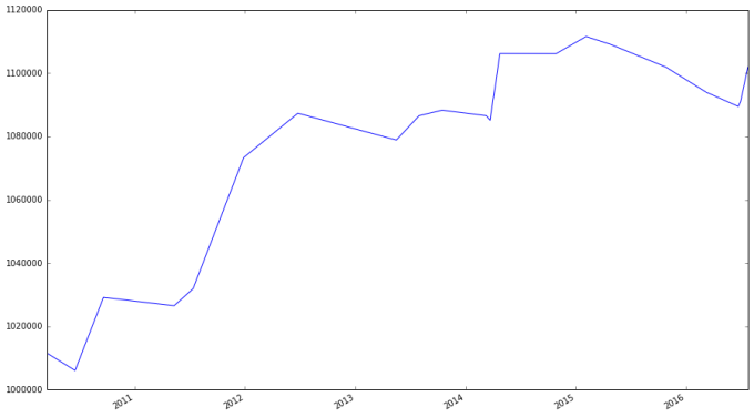
Our portfolio’s value grew by 10% in about six years. Considering that only 10% of the portfolio was ever involved in any single trade, this is not bad performance.

Notice that this strategy never lead to our stop-loss order being triggered. Does this mean we don’t need stop-loss orders? There is no simple answer to this. After all, if we had chosen a different level at which a stop-loss would be triggered, we may have seen it triggered.

Stop-loss orders are automatically triggered and ask no question as to why the order was triggered. This means that both a genuine change in trend or a momentary fluctuation can trigger a stop-loss, with the latter being the more concerning reason since not only do you have to pay for the order, there is no guarantee that you will sell the stock at the price you set, which could make your losses worse. Meanwhile, the trend on which you based your trade still holds, and had the stop-loss not been triggered, you may have made a profit. That said, a stop-loss can help you protect against your own emotions, staying wedded to a trade even though it has lost its value. They’re also good to have if you cannot monitor or quickly access your portfolio, like when you are on vacation.

I have provided links both for and “against” the use of stop-loss orders, but from now on I’m not going to require our backtesting system to account for them. While less realistic (and I do believe an industrial-strength system should account for a stop-loss rule), this simplifies the backtesting task.

A more realistic portfolio would not be betting 10% of its value on only one stock. A more realistic one would consider investing in multiple stocks. Multiple trades may be ongoing at any given time involving multiple companies, and most of the portfolio will be in stocks, not cash. Now that we will be investing in multiple stops and exiting only when moving averages cross (not because of a stop-loss), we will need to change our approach to backtesting. For example, we will be using one pandas DataFrame to contain all buy and sell orders for all stocks being considered, and our loop above will have to track more information.

I have written functions for creating order data for multiple stocks, and a function for performing the backtesting.

def ma_crossover_orders(stocks, fast, slow):
    """
    :param stocks: A list of tuples, the first argument in each tuple being a string containing the ticker symbol of each stock (or however you want the stock represented, so long as it's unique), and the second being a pandas DataFrame containing the stocks, with a "Close" column and indexing by date (like the data frames returned by the Yahoo! Finance API)
    :param fast: Integer for the number of days used in the fast moving average
    :param slow: Integer for the number of days used in the slow moving average

    :return: pandas DataFrame containing stock orders

    This function takes a list of stocks and determines when each stock would be bought or sold depending on a moving average crossover strategy, returning a data frame with information about when the stocks in the portfolio are bought or sold according to the strategy
    """
    fast_str = str(fast) + 'd'
    slow_str = str(slow) + 'd'
    ma_diff_str = fast_str + '-' + slow_str

    trades = pd.DataFrame({"Price": [], "Regime": [], "Signal": []})
    for s in stocks:
        # Get the moving averages, both fast and slow, along with the difference in the moving averages
        s[1][fast_str] = np.round(s[1]["Close"].rolling(window = fast, center = False).mean(), 2)
        s[1][slow_str] = np.round(s[1]["Close"].rolling(window = slow, center = False).mean(), 2)
        s[1][ma_diff_str] = s[1][fast_str] - s[1][slow_str]

        # np.where() is a vectorized if-else function, where a condition is checked for each component of a vector, and the first argument passed is used when the condition holds, and the other passed if it does not
        s[1]["Regime"] = np.where(s[1][ma_diff_str] > 0, 1, 0)
        # We have 1's for bullish regimes and 0's for everything else. Below I replace bearish regimes's values with -1, and to maintain the rest of the vector, the second argument is apple["Regime"]
        s[1]["Regime"] = np.where(s[1][ma_diff_str] < 0, -1, s[1]["Regime"])
        # To ensure that all trades close out, I temporarily change the regime of the last row to 0
        regime_orig = s[1].ix[-1, "Regime"]
        s[1].ix[-1, "Regime"] = 0
        s[1]["Signal"] = np.sign(s[1]["Regime"] - s[1]["Regime"].shift(1))
        # Restore original regime data
        s[1].ix[-1, "Regime"] = regime_orig

        # Get signals
        signals = pd.concat([
            pd.DataFrame({"Price": s[1].loc[s[1]["Signal"] == 1, "Close"],
                         "Regime": s[1].loc[s[1]["Signal"] == 1, "Regime"],
                         "Signal": "Buy"}),
            pd.DataFrame({"Price": s[1].loc[s[1]["Signal"] == -1, "Close"],
                         "Regime": s[1].loc[s[1]["Signal"] == -1, "Regime"],
                         "Signal": "Sell"}),
        ])
        signals.index = pd.MultiIndex.from_product([signals.index, [s[0]]], names = ["Date", "Symbol"])
        trades = trades.append(signals)

    trades.sort_index(inplace = True)
    trades.index = pd.MultiIndex.from_tuples(trades.index, names = ["Date", "Symbol"])

    return trades


def backtest(signals, cash, port_value = .1, batch = 100):
    """
    :param signals: pandas DataFrame containing buy and sell signals with stock prices and symbols, like that returned by ma_crossover_orders
    :param cash: integer for starting cash value
    :param port_value: maximum proportion of portfolio to risk on any single trade
    :param batch: Trading batch sizes

    :return: pandas DataFrame with backtesting results

    This function backtests strategies, with the signals generated by the strategies being passed in the signals DataFrame. A fictitious portfolio is simulated and the returns generated by this portfolio are reported.
    """

    SYMBOL = 1 # Constant for which element in index represents symbol
    portfolio = dict()    # Will contain how many stocks are in the portfolio for a given symbol
    port_prices = dict()  # Tracks old trade prices for determining profits
    # Dataframe that will contain backtesting report
    results = pd.DataFrame({"Start Cash": [],
                            "End Cash": [],
                            "Portfolio Value": [],
                            "Type": [],
                            "Shares": [],
                            "Share Price": [],
                            "Trade Value": [],
                            "Profit per Share": [],
                            "Total Profit": []})

    for index, row in signals.iterrows():
        # These first few lines are done for any trade
        shares = portfolio.setdefault(index[SYMBOL], 0)
        trade_val = 0
        batches = 0
        cash_change = row["Price"] * shares   # Shares could potentially be a positive or negative number (cash_change will be added in the end; negative shares indicate a short)
        portfolio[index[SYMBOL]] = 0  # For a given symbol, a position is effectively cleared

        old_price = port_prices.setdefault(index[SYMBOL], row["Price"])
        portfolio_val = 0
        for key, val in portfolio.items():
            portfolio_val += val * port_prices[key]

        if row["Signal"] == "Buy" and row["Regime"] == 1:  # Entering a long position
            batches = np.floor((portfolio_val + cash) * port_value) // np.ceil(batch * row["Price"]) # Maximum number of batches of stocks invested in
            trade_val = batches * batch * row["Price"] # How much money is put on the line with each trade
            cash_change -= trade_val  # We are buying shares so cash will go down
            portfolio[index[SYMBOL]] = batches * batch  # Recording how many shares are currently invested in the stock
            port_prices[index[SYMBOL]] = row["Price"]   # Record price
            old_price = row["Price"]
        elif row["Signal"] == "Sell" and row["Regime"] == -1: # Entering a short
            pass
            # Do nothing; can we provide a method for shorting the market?
        #else:
            #raise ValueError("I don't know what to do with signal " + row["Signal"])

        pprofit = row["Price"] - old_price   # Compute profit per share; old_price is set in such a way that entering a position results in a profit of zero

        # Update report
        results = results.append(pd.DataFrame({
                "Start Cash": cash,
                "End Cash": cash + cash_change,
                "Portfolio Value": cash + cash_change + portfolio_val + trade_val,
                "Type": row["Signal"],
                "Shares": batch * batches,
                "Share Price": row["Price"],
                "Trade Value": abs(cash_change),
                "Profit per Share": pprofit,
                "Total Profit": batches * batch * pprofit
            }, index = [index]))
        cash += cash_change  # Final change to cash balance

    results.sort_index(inplace = True)
    results.index = pd.MultiIndex.from_tuples(results.index, names = ["Date", "Symbol"])

    return results

# Get more stocks
microsoft = web.DataReader("MSFT", "yahoo", start, end)
google = web.DataReader("GOOG", "yahoo", start, end)
facebook = web.DataReader("FB", "yahoo", start, end)
twitter = web.DataReader("TWTR", "yahoo", start, end)
netflix = web.DataReader("NFLX", "yahoo", start, end)
amazon = web.DataReader("AMZN", "yahoo", start, end)
yahoo = web.DataReader("YHOO", "yahoo", start, end)
sony = web.DataReader("SNY", "yahoo", start, end)
nintendo = web.DataReader("NTDOY", "yahoo", start, end)
ibm = web.DataReader("IBM", "yahoo", start, end)
hp = web.DataReader("HPQ", "yahoo", start, end)

signals = ma_crossover_orders([("AAPL", ohlc_adj(apple)),
                              ("MSFT",  ohlc_adj(microsoft)),
                              ("GOOG",  ohlc_adj(google)),
                              ("FB",    ohlc_adj(facebook)),
                              ("TWTR",  ohlc_adj(twitter)),
                              ("NFLX",  ohlc_adj(netflix)),
                              ("AMZN",  ohlc_adj(amazon)),
                              ("YHOO",  ohlc_adj(yahoo)),
                              ("SNY",   ohlc_adj(yahoo)),
                              ("NTDOY", ohlc_adj(nintendo)),
                              ("IBM",   ohlc_adj(ibm)),
                              ("HPQ",   ohlc_adj(hp))],
                            fast = 20, slow = 50)
signals

		Price	Regime	Signal
Date	Symbol
2010-03-16	AAPL	29.355667	1.0	Buy
	AMZN	131.789993	1.0	Buy
	GOOG	282.318173	-1.0	Sell
	HPQ	20.722316	1.0	Buy
	IBM	110.563240	1.0	Buy
	MSFT	24.677580	-1.0	Sell
	NFLX	10.090000	1.0	Buy
	NTDOY	37.099998	1.0	Buy
	SNY	16.360001	-1.0	Sell
	YHOO	16.360001	-1.0	Sell
2010-03-17	SNY	16.500000	1.0	Buy
	YHOO	16.500000	1.0	Buy
2010-03-22	GOOG	278.472004	1.0	Buy
2010-03-23	MSFT	25.106096	1.0	Buy
2010-05-03	GOOG	265.035411	-1.0	Sell
2010-05-10	HPQ	19.435830	-1.0	Sell
2010-05-14	NTDOY	35.799999	-1.0	Sell
2010-05-17	SNY	16.270000	-1.0	Sell
	YHOO	16.270000	-1.0	Sell
2010-05-19	AMZN	124.589996	-1.0	Sell
	MSFT	23.835187	-1.0	Sell
2010-05-21	IBM	108.322991	-1.0	Sell
2010-06-10	AAPL	32.764038	0.0	Sell
2010-06-11	AAPL	33.156405	-1.0	Sell
2010-06-18	AAPL	35.845436	1.0	Buy
2010-06-28	IBM	111.397697	1.0	Buy
2010-07-01	IBM	105.861499	-1.0	Sell
2010-07-06	IBM	106.630175	1.0	Buy
2010-07-09	NTDOY	36.950001	1.0	Buy
2010-07-20	IBM	109.298956	-1.0	Sell
…	…	…	…	…
2016-06-23	AAPL	95.582210	1.0	Buy
	TWTR	17.040001	1.0	Buy
2016-06-27	AAPL	91.544087	-1.0	Sell
	FB	108.970001	-1.0	Sell
2016-06-28	SNY	36.040001	-1.0	Sell
	YHOO	36.040001	-1.0	Sell
2016-06-30	AAPL	95.084904	1.0	Buy
	NFLX	91.480003	0.0	Sell
2016-07-01	NFLX	96.669998	-1.0	Sell
	SNY	37.990002	1.0	Buy
	YHOO	37.990002	1.0	Buy
2016-07-11	AAPL	96.457473	-1.0	Sell
	NTDOY	27.700001	1.0	Buy
2016-07-14	MSFT	53.407133	1.0	Buy
2016-07-25	AAPL	96.815526	1.0	Buy
	FB	121.629997	1.0	Buy
2016-07-26	GOOG	738.419983	1.0	Buy
2016-08-18	NFLX	96.160004	1.0	Buy
2016-09-01	AAPL	106.730003	1.0	Sell
2016-09-02	AMZN	772.440002	1.0	Sell
	FB	126.510002	1.0	Sell
	GOOG	771.460022	1.0	Sell
	HPQ	14.490000	1.0	Sell
	IBM	159.550003	1.0	Sell
	MSFT	57.669998	1.0	Sell
	NFLX	97.379997	1.0	Sell
	NTDOY	28.840000	1.0	Sell
	SNY	43.279999	1.0	Sell
	TWTR	19.549999	1.0	Sell
	YHOO	43.279999	1.0	Sell

475 rows × 3 columns

bk = backtest(signals, 1000000)
bk

		End Cash	Portfolio Value	Profit per Share	Share Price	Shares	Start Cash	Total Profit	Trade Value	Type
Date	Symbol
2010-03-16	AAPL	9.001907e+05	1.000000e+06	0.000000	29.355667	3400.0	1.000000e+06	0.0	99809.2678	Buy
	AMZN	8.079377e+05	1.000000e+06	0.000000	131.789993	700.0	9.001907e+05	0.0	92252.9951	Buy
	GOOG	8.079377e+05	1.000000e+06	0.000000	282.318173	0.0	8.079377e+05	0.0	0.0000	Sell
	HPQ	7.084706e+05	1.000000e+06	0.000000	20.722316	4800.0	8.079377e+05	0.0	99467.1168	Buy
	IBM	6.089637e+05	1.000000e+06	0.000000	110.563240	900.0	7.084706e+05	0.0	99506.9160	Buy
	MSFT	6.089637e+05	1.000000e+06	0.000000	24.677580	0.0	6.089637e+05	0.0	0.0000	Sell
	NFLX	5.090727e+05	1.000000e+06	0.000000	10.090000	9900.0	6.089637e+05	0.0	99891.0000	Buy
	NTDOY	4.126127e+05	1.000000e+06	0.000000	37.099998	2600.0	5.090727e+05	0.0	96459.9948	Buy
	SNY	4.126127e+05	1.000000e+06	0.000000	16.360001	0.0	4.126127e+05	0.0	0.0000	Sell
	YHOO	4.126127e+05	1.000000e+06	0.000000	16.360001	0.0	4.126127e+05	0.0	0.0000	Sell
2010-03-17	SNY	3.136127e+05	1.000000e+06	0.000000	16.500000	6000.0	4.126127e+05	0.0	99000.0000	Buy
	YHOO	2.146127e+05	1.000000e+06	0.000000	16.500000	6000.0	3.136127e+05	0.0	99000.0000	Buy
2010-03-22	GOOG	1.310711e+05	1.000000e+06	0.000000	278.472004	300.0	2.146127e+05	0.0	83541.6012	Buy
2010-03-23	MSFT	3.315733e+04	1.000000e+06	0.000000	25.106096	3900.0	1.310711e+05	0.0	97913.7744	Buy
2010-05-03	GOOG	1.126680e+05	9.959690e+05	-13.436593	265.035411	0.0	3.315733e+04	-0.0	79510.6233	Sell
2010-05-10	HPQ	2.059599e+05	9.897939e+05	-1.286486	19.435830	0.0	1.126680e+05	-0.0	93291.9840	Sell
2010-05-14	NTDOY	2.990399e+05	9.864139e+05	-1.299999	35.799999	0.0	2.059599e+05	-0.0	93079.9974	Sell
2010-05-17	SNY	3.966599e+05	9.850339e+05	-0.230000	16.270000	0.0	2.990399e+05	-0.0	97620.0000	Sell
	YHOO	4.942799e+05	9.836539e+05	-0.230000	16.270000	0.0	3.966599e+05	-0.0	97620.0000	Sell
2010-05-19	AMZN	5.814929e+05	9.786139e+05	-7.199997	124.589996	0.0	4.942799e+05	-0.0	87212.9972	Sell
	MSFT	6.744502e+05	9.736573e+05	-1.270909	23.835187	0.0	5.814929e+05	-0.0	92957.2293	Sell
2010-05-21	IBM	7.719409e+05	9.716411e+05	-2.240249	108.322991	0.0	6.744502e+05	-0.0	97490.6919	Sell
2010-06-10	AAPL	8.833386e+05	9.832296e+05	3.408371	32.764038	0.0	7.719409e+05	0.0	111397.7292	Sell
2010-06-11	AAPL	8.833386e+05	9.832296e+05	3.800738	33.156405	0.0	8.833386e+05	0.0	0.0000	Sell
2010-06-18	AAPL	7.865559e+05	9.832296e+05	0.000000	35.845436	2700.0	8.833386e+05	0.0	96782.6772	Buy
2010-06-28	IBM	6.974378e+05	9.832296e+05	0.000000	111.397697	800.0	7.865559e+05	0.0	89118.1576	Buy
2010-07-01	IBM	7.821270e+05	9.788006e+05	-5.536198	105.861499	0.0	6.974378e+05	-0.0	84689.1992	Sell
2010-07-06	IBM	6.861598e+05	9.788006e+05	0.000000	106.630175	900.0	7.821270e+05	0.0	95967.1575	Buy
2010-07-09	NTDOY	5.900898e+05	9.788006e+05	0.000000	36.950001	2600.0	6.861598e+05	0.0	96070.0026	Buy
2010-07-20	IBM	6.884589e+05	9.812025e+05	2.668781	109.298956	0.0	5.900898e+05	0.0	98369.0604	Sell
…	…	…	…	…	…	…	…	…	…	…
2016-06-23	AAPL	3.951693e+05	1.863808e+06	0.000000	95.582210	1900.0	5.767755e+05	0.0	181606.1990	Buy
	TWTR	2.094333e+05	1.863808e+06	0.000000	17.040001	10900.0	3.951693e+05	0.0	185736.0109	Buy
2016-06-27	AAPL	3.833670e+05	1.856135e+06	-4.038123	91.544087	0.0	2.094333e+05	-0.0	173933.7653	Sell
	FB	5.795130e+05	1.862921e+06	3.770004	108.970001	0.0	3.833670e+05	0.0	196146.0018	Sell
2016-06-28	SNY	7.885450e+05	1.880959e+06	3.110001	36.040001	0.0	5.795130e+05	0.0	209032.0058	Sell
	YHOO	9.975770e+05	1.898997e+06	3.110001	36.040001	0.0	7.885450e+05	0.0	209032.0058	Sell
2016-06-30	AAPL	8.169157e+05	1.898997e+06	0.000000	95.084904	1900.0	9.975770e+05	0.0	180661.3176	Buy
	NFLX	9.907277e+05	1.893981e+06	-2.640000	91.480003	0.0	8.169157e+05	-0.0	173812.0057	Sell
2016-07-01	NFLX	9.907277e+05	1.893981e+06	2.549995	96.669998	0.0	9.907277e+05	0.0	0.0000	Sell
	SNY	8.045767e+05	1.893981e+06	0.000000	37.990002	4900.0	9.907277e+05	0.0	186151.0098	Buy
	YHOO	6.184257e+05	1.893981e+06	0.000000	37.990002	4900.0	8.045767e+05	0.0	186151.0098	Buy
2016-07-11	AAPL	8.016949e+05	1.896589e+06	1.372569	96.457473	0.0	6.184257e+05	0.0	183269.1987	Sell
	NTDOY	6.133349e+05	1.896589e+06	0.000000	27.700001	6800.0	8.016949e+05	0.0	188360.0068	Buy
2016-07-14	MSFT	4.264099e+05	1.896589e+06	0.000000	53.407133	3500.0	6.133349e+05	0.0	186924.9655	Buy
2016-07-25	AAPL	2.424604e+05	1.896589e+06	0.000000	96.815526	1900.0	4.264099e+05	0.0	183949.4994	Buy
	FB	6.001543e+04	1.896589e+06	0.000000	121.629997	1500.0	2.424604e+05	0.0	182444.9955	Buy
2016-07-26	GOOG	-8.766857e+04	1.896589e+06	0.000000	738.419983	200.0	6.001543e+04	0.0	147683.9966	Buy
2016-08-18	NFLX	-2.703726e+05	1.896589e+06	0.000000	96.160004	1900.0	-8.766857e+04	0.0	182704.0076	Buy
2016-09-01	AAPL	-6.758557e+04	1.915427e+06	9.914477	106.730003	0.0	-2.703726e+05	0.0	202787.0057	Sell
2016-09-02	AMZN	1.641464e+05	1.979327e+06	213.000000	772.440002	0.0	-6.758557e+04	0.0	231732.0006	Sell
	FB	3.539114e+05	1.986647e+06	4.880005	126.510002	0.0	1.641464e+05	0.0	189765.0030	Sell
	GOOG	5.082034e+05	1.993255e+06	33.040039	771.460022	0.0	3.539114e+05	0.0	154292.0044	Sell
	HPQ	7.081654e+05	2.006030e+06	0.925746	14.490000	0.0	5.082034e+05	0.0	199962.0000	Sell
	IBM	8.996254e+05	2.015652e+06	8.018727	159.550003	0.0	7.081654e+05	0.0	191460.0036	Sell
	MSFT	1.101470e+06	2.030572e+06	4.262865	57.669998	0.0	8.996254e+05	0.0	201844.9930	Sell
	NFLX	1.286492e+06	2.032890e+06	1.219993	97.379997	0.0	1.101470e+06	0.0	185021.9943	Sell
	NTDOY	1.482604e+06	2.040642e+06	1.139999	28.840000	0.0	1.286492e+06	0.0	196112.0000	Sell
	SNY	1.694676e+06	2.066563e+06	5.289997	43.279999	0.0	1.482604e+06	0.0	212071.9951	Sell
	TWTR	1.907771e+06	2.093922e+06	2.509998	19.549999	0.0	1.694676e+06	0.0	213094.9891	Sell
	YHOO	2.119843e+06	2.119843e+06	5.289997	43.279999	0.0	1.907771e+06	0.0	212071.9951	Sell

475 rows × 9 columns

bk["Portfolio Value"].groupby(level = 0).apply(lambda x: x[-1]).plot()

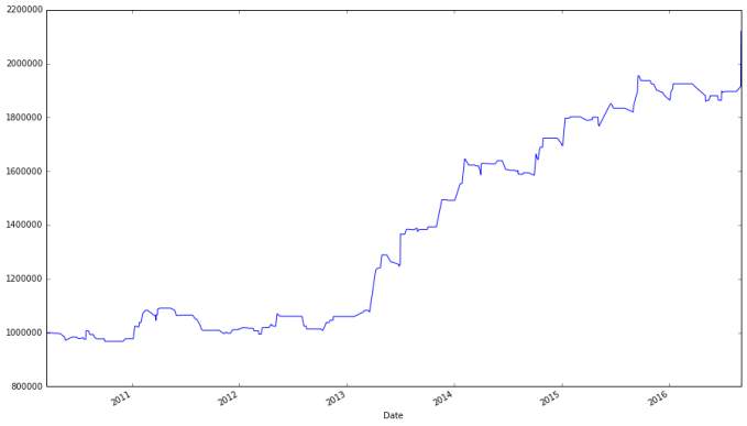
A more realistic portfolio that can invest in any in a list of twelve (tech) stocks has a final growth of about 100%. How good is this? While on the surface not bad, we will see we could have done better.

Benchmarking

Backtesting is only part of evaluating the efficacy of a trading strategy. We would like to benchmark the strategy, or compare it to other available (usually well-known) strategies in order to determine how well we have done.

Whenever you evaluate a trading system, there is one strategy that you should always check, one that beats all but a handful of managed mutual funds and investment managers: buy and hold SPY. The efficient market hypothesis claims that it is all but impossible for anyone to beat the market. Thus, one should always buy an index fund that merely reflects the composition of the market. SPY is an exchange-traded fund (a mutual fund that is traded on the market like a stock) whose value effectively represents the value of the stocks in the S&P 500 stock index. By buying and holding SPY, we are effectively trying to match our returns with the market rather than beat it.

I obtain data on SPY below, and look at the profits for simply buying and holding SPY.

spyder = web.DataReader("SPY", "yahoo", start, end)
spyder.iloc[[0,-1],:]

	Open	High	Low	Close	Volume	Adj Close
Date
2010-01-04	112.370003	113.389999	111.510002	113.330002	118944600	99.292299
2016-09-01	217.369995	217.729996	216.029999	217.389999	93859000	217.389999

batches = 1000000 // np.ceil(100 * spyder.ix[0,"Adj Close"]) # Maximum number of batches of stocks invested in
trade_val = batches * batch * spyder.ix[0,"Adj Close"] # How much money is used to buy SPY
final_val = batches * batch * spyder.ix[-1,"Adj Close"] + (1000000 - trade_val) # Final value of the portfolio
final_val

2180977.0

# We see that the buy-and-hold strategy beats the strategy we developed earlier. I would also like to see a plot.
ax_bench = (spyder["Adj Close"] / spyder.ix[0, "Adj Close"]).plot(label = "SPY")
ax_bench = (bk["Portfolio Value"].groupby(level = 0).apply(lambda x: x[-1]) / 1000000).plot(ax = ax_bench, label = "Portfolio")
ax_bench.legend(ax_bench.get_lines(), [l.get_label() for l in ax_bench.get_lines()], loc = 'best')
ax_bench

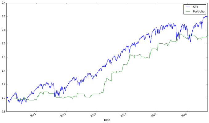
Buying and holding SPY beats our trading system, at least how we currently set it up, and we haven’t even accounted for how expensive our more complex strategy is in terms of fees. Given both the opportunity cost and the expense associated with the active strategy, we should not use it.

What could we do to improve the performance of our system? For starters, we could try diversifying. All the stocks we considered were tech companies, which means that if the tech industry is doing poorly, our portfolio will reflect that. We could try developing a system that can also short stocks or bet bearishly, so we can take advantage of movement in any direction. We could seek means for forecasting how high we expect a stock to move. Whatever we do, though, must beat this benchmark; otherwise there is an opportunity cost associated with our trading system.

Other benchmark strategies exist, and if our trading system beat the “buy and hold SPY” strategy, we may check against them. Some such strategies include:

• Buy SPY when its closing monthly price is aboves its ten-month moving average.
• Buy SPY when its ten-month momentum is positive. (Momentum is the first difference of a moving average process, or .)

(I first read of these strategies here.) The general lesson still holds: don’t use a complex trading system with lots of active trading when a simple strategy involving an index fund without frequent trading beats it. This is actually a very difficult requirement to meet.

As a final note, suppose that your trading system did manage to beat any baseline strategy thrown at it in backtesting. Does backtesting predict future performance? Not at all. Backtesting has a propensity for overfitting, so just because backtesting predicts high growth doesn’t mean that growth will hold in the future.

Conclusion

While this lecture ends on a depressing note, keep in mind that the efficient market hypothesis has many critics. My own opinion is that as trading becomes more algorithmic, beating the market will become more difficult. That said, it may be possible to beat the market, even though mutual funds seem incapable of doing so (bear in mind, though, that part of the reason mutual funds perform so poorly is because of fees, which is not a concern for index funds).

This lecture is very brief, covering only one type of strategy: strategies based on moving averages. Many other trading signals exist and employed. Additionally, we never discussed in depth shorting stocks, currency trading, or stock options. Stock options, in particular, are a rich subject that offer many different ways to bet on the direction of a stock. You can read more about derivatives (including stock options and other derivatives) in the book Derivatives Analytics with Python: Data Analysis, Models, Simulation, Calibration and Hedging, which is available from the University of Utah library (for University of Utah students).

Another resource (which I used as a reference while writing this lecture) is the O’Reilly book Python for Finance, also available from the University of Utah library.

Remember that it is possible (if not common) to lose money in the stock market. It’s also true, though, that it’s difficult to find returns like those found in stocks, and any investment strategy should take investing in it seriously. This lecture is intended to provide a starting point for evaluating stock trading and investment, and I hope you continue to explore these ideas.

Problems

Problem 1

Devise a trading strategy as described in lecture based on moving-average crossovers (you do not need a stop-loss). Pick a list of at least 15 stocks that have existed since January 1st, 2010. Backtest your strategy with the stocks chosen and benchmark the performance of your portfolio against the performance of SPY. Are you able to beat the market?

Problem 2

Realistically, with every trade a commission is applied. Read about how commission works, and modify the backtest() function in the lecture to allow multiple commission structures (flat fee, percentage of portfolio, etc.) to be simulated.

Additionally, our current moving average crossover strategy results in a trading signal triggering the moment two moving averages cross. We would like to make sure signals are more robust, either by:

1. Triggering a trade when the moving averages differ by a fixed amount
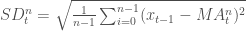
2. Triggering a trade when the moving averages differ by some amount of (rolling) standard deviations, which are defined by:

(pandas does have means for computing rolling standard deviations.) Regarding the latter, if the moving averages differ by , a trading signal is sent. Modify the function ma_crossover_orders() so that these restrictions can be implemented. Specifically, you should have the ability to set how many days are in the window of the rolling standard deviation (it need not be the same as either the fast or slow moving average windows), and how many standard deviations the moving averages must differ by in order for a signal to be sent. (The current behavior of these functions should still be possible; in fact, it should be the default behavior.)

Once these changes have been made, repeat problem 1, including a realistic commission scheme (consider looking up one from a brokerage firm) when simulating the performance of the portfolio, and requiring the moving averages differ by some fixed number or standard deviations in order for signals to be sent.

Problem 3

We did not set up our trading system to allow for shorting stocks. Short selling is much trickier, since losses from short selling are unlimited (a long position, on the other hand, limits losses to the total value of the assets purchased). Read about short selling here. Then modify the function backtest() to allow for short selling. How will the function decide how to conduct short sales, including how many shares to short and how to account for shorted stocks when conducting other trades? We leave this up to you to decide. As a hint, the number of shares being shorted can be represented internally in the function by a negative number.

Once this is done, repeat Problem 1, perhaps also using features implemented in Problem 2.

---

I have created a video course published by Packt Publishing entitled Training Your Systems with Python Statistical Modeling, the third volume in a four-volume set of video courses entitled, Taming Data with Python; Excelling as a Data Analyst. This course discusses how to use Python for machine learning. The course covers classical statistical methods, supervised learning including classification and regression, clustering, dimensionality reduction, and more! The course is peppered with examples demonstrating the techniques and software on real-world data and visuals to explain the concepts presented. Viewers get a hands-on experience using Python for machine learning. If you are starting out using Python for data analysis or know someone who is, please consider buying my course or at least spreading the word about it. You can buy the course directly or purchase a subscription to Mapt and watch it there.

If you like my blog and would like to support it, spread the word (if not get a copy yourself)! Also, stay tuned for future courses I publish with Packt at the Video Courses section of my site.

Advertisement