
A few weeks ago, I ranted about the R backtesting package quantstrat and its related packages. Specifically, I disliked that I would not be able to do a particular type of walk-forward analysis with quantstrat, or at least was not able to figure out how to do so. In general, I disliked how usable quantstrat seemed to be. The package’s interface seems flexible in some areas, inflexible in others, due to a strange architecture that I eventually was not willing to put up with anymore.
I got good responses from people both agreeing and disagreeing with me, and R users who did not want me to stop writing about R. In comments on Reddit and on my post directly (by my invitation), Ilya Kipnis argued that while quantstrat‘s learning curve is steep, it adopts the architecture and algorithms it uses for good reasons, being designed for use by quants in large hedgefunds with varying data challenges. He recommended that, instead of abandoning the package, I should look for more help, particularly from R’s R-SIG-Finance mailing list. One of quantstrat‘s contributors, Joshua Ulrich, directed me in the comments of my blog to what appears to be an experimental alternative quantstrat architecture, using the object-oriented framework provided in R6, which I was not aware of and, I think, looks like a promising alternative to the current architecture. Meanwhile, other users mentioned the quality of packages like PerformanceAnalytics and R’s excellent time series functionality (which I use heavily in my work as a Ph.D. student). Some just wanted me to keep writing about R for finance since they cannot make the switch to Python.
Given those comments and a personal bias towards R, I cannot envision myself completely divorcing myself from R. I’m going to try and develop a much simpler project demonstrating basic walk.forward() usage. I ran into difficulties trying to get any example of walk-forward analysis working (either with or without using walk.forward()) and I described my difficulties on the R-SIG-Finance mailing list last week. Perhaps someone will understand what I’m trying to accomplish and will tell me the best way to accomplish that task (I have yet to hear from anyone).
Nevertheless, while the experimental object-oriented architecture I saw looks promising, my complaints about quantstrat‘s architecture stand, Mr. Kipnis’s defense notwithstanding. I believe there is a better way to design a backtesting package.
I should also mention that despite having published my lecture on stock data analysis with Python on my website about nine months ago, those articles account for the vast majority of traffic to this blog. In addition, there are people requesting that I create (paid-for) content on Python for finance. Clearly, the demand for my Python content is higher than the demand for my R content, even though I have written a lot more about R and, personally, am more fluent in R. (R is the language I use for my own “work” and my preferred language for certain projects.) Given this, it’s time I start exploring Python for finance more than I already have.
Thus, cue backtrader. This is the first article where I explore the package, but I have been looking through its documentation for some time and have yet to be completely disappointed, though it is not perfect. It heavily uses an object-oriented approach–which, in all honesty, seems natural for backtesting–and seems capable of doing what quantstrat does, yet looks flexible. The features for creating strategies, backtesting, data management (I like the idea of data feeds), designing commission structures and accounting for slippage, logging, and more, have impressed me. In fact, there’s functionality to connect to a brokerage for live trading! I’m still getting over the fact that the package, unlike quantstrat, appears to be well-documented.
The only feature that, to me, appears to be a glaring omission, is the ability to log results to a pandas DataFrame. pandas was designed to handle time series, and is in general an essential package to Python data analysis, in my opinion. backtrader‘s closest Python “competitor”, zipline, advertises its strong pandas support (though Mr. Kipnis believes it is inferior to quantstrat and looking though the documentation it has not bedazzled me to the extent backtrader has). There is a likely work-around, though; backtrader‘s logging functionality allows logging to files, including CSV files, so a user can perform a backtest, define what metrics she wants captured in a CSV file, then read that file into a pandas DataFrame. It would be nice to cut out the middle-man, though.
I also am not seeing anywhere in backtrader how I could perform the walk-forward analysis I want to perform. Having said that, what I want to do should not be complicated! In fact, I should not need a built-in function for walk-forward analysis. I should be able to tell a backtester which dates I want to use for training, which I want to use for testing, and then run lots of these tests in batch. I could spam objects for backtesting, giving each one unique training-testing periods, then look at their end results. This looks achievable with backtrader, while I was struggling to do this with quantstrat (I even tried a hideous for loop, and it didn’t work for mysterious reasons).
I’m not going to worry about walk-forward analysis now, though. I’m more concerned with getting started. In this post, I will re-develop the strategy I had written in my article on Python for backtesting, and add features like those I added when using quantstrat, such as accounting for transaction costs.
Unfortunately, I doubt I will be able to replicate the results seen in either my Python posts or my quantstrat posts. Yahoo! Finance made changes to their API that changed their data, arguably for worse. I have not yet explored alternatives to Yahoo! Finance, but for now I’m okay with that. I’m more interested in making the software and packages do what I want than developing good trading strategies.
Developing the Strategy
backtrader takes an object-oriented approach to backtesting. Users define objects representing important aspects of the backtesting system, such as the trading strategy, the broker, and sizers. These modules can then be put together, allowing for more flexible analysis.
Let’s first load in needed libraries.
import backtrader as bt
import backtrader.indicators as btind
import datetime
import pandas as pd
from pandas import Series, DataFrame
import random
from copy import deepcopy
I first define a strategy object. I’m looking at a simple moving average crossover strategy that I call SMAC. Strategy development in backtrader is more involved than it is with quantstrat. Users need to define more, such as how data sets (such as stock symbols) should be handled. In fact, it feels as if users need to write important parts of the loop that in quantstrat are already programmed in.
This is not a bad thing, in my opinion. One of my complaints with quantstrat was that I felt wedded to however the system was processing trades and signals in its loop, whether I liked that approach or not.
For example, it would process each symbol separately, and I did not like that; I wanted a backtester that would behave like I as a trader would, looking to the account to see if there is enough money for a trade accounting for the cash gone due to other trades. Ilya Kipnis on Reddit responded that this is done because a hedge fund always ensures there’s enough cash to place a trade should it be needed, but I am not a hedge fund. I’m a poor graduate student considering live trading with a pitiful, \$100 account just for the sake of the experience (and I feel guilty about putting that much money on the line). Money management is very important to me, I’m cheap, and I don’t like cutting corners.
In other situations I might have been able to make it do what I want but only after looking closely at the loop’s source code, and coming up with what felt like a hack to do what I wanted. For example, I wanted to be sizing trades so each would correspond to having a value of roughly 10% of the value of the account at that instant. I had to closely inspect the loop to see how to do this, and given that I misunderstood what the loop was doing, I think the solution I wrote was incorrect.
By defining important parts of the loop myself, I’m given greater flexibility and have fewer opportunities for confusion; I know what’s going on because I wrote it myself. The cost is the strategy is less readable and more time needs to be invested in the beginning to get an initial backtest, but I am not bothered by this.
To define a strategy, I need to write an __init__() method that defines important indicators and initializes certain aspects (for example, I needed to use the method _addobserver() for tracking buying and selling in the plot I wanted). Then I define a next() method that will be called at each bar in the backtest. In this example next() will only be responsible for sending “buy” and “sell” orders (working at market; I’m not worrying about order types right now). A more sophisticated system may see a log() method defined for logging results and next() calling logging functions. I’m not worried about logging right now, though, so this is good enough.
Unlike with quantstrat, you need to tell your strategy how to handle multiple symbols (all of them independent data feeds). It will not automatically apply the strategy to every symbol in the data feed. In this case, I loop through every data feed available to the strategy by name (they are all stock symbols, but you could imagine setting up a system where one of the data feeds is some fundamental indicator, like the economy’s unemployment rate). In __init__(), I compute some indicators (simple moving averages in this case) and store them in dictionaries indexed by the names of the data feeds. Then, in next()‘s loop, I check whether a crossover of the fast and slow moving averages has taken place, which may trigger a buy() or sell() signal depending on the context. (I also need to check whether I currently have a position for that symbol since my strategy does not increase or decrease a position; it only enters or exits.) If a signal has been generated, I buy or sell the symbol in question. (I got a lot of help figuring this out from this blog post on backtrader‘s official blog.)
The very first line is a dict called params that will be added to the object as an attribute. This provides a means for generalizing a strategy. In this case, we can change the window size of the fast and slow moving averages. I did this in two ways, since I use the strategy in two different contexts. In one, I backtest in a one-off manner. In another, I use it in optimization, and in the latter scenario I want these parameters passed as a tuple (since I generate possible combinations as tuples. I include an optim parameter to toggle whether to use the tuple-based format or not, but in general optim is turned on when I am optimizing the strategy and I want alternative functionality.
The strategy is defined below.
class SMAC(bt.Strategy):
    """A simple moving average crossover strategy; crossing of a fast and slow moving average generates buy/sell
       signals"""
    params = {"fast": 20, "slow": 50,                  # The windows for both fast and slow moving averages
              "optim": False, "optim_fs": (20, 50)}    # Used for optimization; equivalent of fast and slow, but a tuple
                                                       # The first number in the tuple is the fast MA's window, the
                                                       # second the slow MA's window

    def __init__(self):
        """Initialize the strategy"""

        self.fastma = dict()
        self.slowma = dict()
        self.regime = dict()

        self._addobserver(True, bt.observers.BuySell)    # CAUTION: Abuse of the method, I will change this in future code (see: https://community.backtrader.com/topic/473/plotting-just-the-account-s-value/4)

        if self.params.optim:    # Use a tuple during optimization
            self.params.fast, self.params.slow = self.params.optim_fs    # fast and slow replaced by tuple's contents

        if self.params.fast > self.params.slow:
            raise ValueError(
                "A SMAC strategy cannot have the fast moving average's window be " + \
                 "greater than the slow moving average window.")

        for d in self.getdatanames():

            # The moving averages
            self.fastma[d] = btind.SimpleMovingAverage(self.getdatabyname(d),      # The symbol for the moving average
                                                       period=self.params.fast,    # Fast moving average
                                                       plotname="FastMA: " + d)
            self.slowma[d] = btind.SimpleMovingAverage(self.getdatabyname(d),      # The symbol for the moving average
                                                       period=self.params.slow,    # Slow moving average
                                                       plotname="SlowMA: " + d)

            # Get the regime
            self.regime[d] = self.fastma[d] - self.slowma[d]    # Positive when bullish

    def next(self):
        """Define what will be done in a single step, including creating and closing trades"""
        for d in self.getdatanames():    # Looping through all symbols
            pos = self.getpositionbyname(d).size or 0
            if pos == 0:    # Are we out of the market?
                # Consider the possibility of entrance
                # Notice the indexing; [0] always mens the present bar, and [-1] the bar immediately preceding
                # Thus, the condition below translates to: "If today the regime is bullish (greater than
                # 0) and yesterday the regime was not bullish"
                if self.regime[d][0] > 0 and self.regime[d][-1] <= 0:    # A buy signal
                    self.buy(data=self.getdatabyname(d))

            else:    # We have an open position
                if self.regime[d][0] <= 0 and self.regime[d][-1] > 0:    # A sell signal
                    self.sell(data=self.getdatabyname(d))
After defining the strategy, I define a sizing object, called a Sizer, responsible for determining how many shares to purchase or how many to sell in a trade. For my strategy, I only enter or exit positions, and when I enter a position, I want it to be worth roughly 10% of the portfolio at the time. I also require trades be done in batches of 100 shares. There are two parameters in my sizer, prop and batch, that can alter the numbers involved in this strategy.
class PropSizer(bt.Sizer):
    """A position sizer that will buy as many stocks as necessary for a certain proportion of the portfolio
       to be committed to the position, while allowing stocks to be bought in batches (say, 100)"""
    params = {"prop": 0.1, "batch": 100}

    def _getsizing(self, comminfo, cash, data, isbuy):
        """Returns the proper sizing"""

        if isbuy:    # Buying
            target = self.broker.getvalue() * self.params.prop    # Ideal total value of the position
            price = data.close[0]
            shares_ideal = target / price    # How many shares are needed to get target
            batches = int(shares_ideal / self.params.batch)    # How many batches is this trade?
            shares = batches * self.params.batch    # The actual number of shares bought

            if shares * price > cash:
                return 0    # Not enough money for this trade
            else:
                return shares

        else:    # Selling
            return self.broker.getposition(data).size    # Clear the position
Getting Cerebral with Cerebro
A Cerebro object is the conductor of your backtest and analysis. The object manages data, strategies, accounts, data collectors, and other aspects. It’s responsible for running the backtest, offering analytics, and creating requested plots. Below I create one for our first run of the strategy.
cerebro = bt.Cerebro(stdstats=False) # I don't want the default plot objects
Let’s first get some money and give it to our “broker”. I also assign a 2% commission to the broker.
cerebro.broker.set_cash(1000000)    # Set our starting cash to $1,000,000
cerebro.broker.setcommission(0.02)
We obviously can’t backtest without data. backtrader views data as a feed, which is a file or object that gives data to the Cerebro object, which reacts to that data. These feeds can be pandas DataFrames, CSV files, databases, even live data streams.
Here I add data for multiple symbols to the Cerebro object, all presumably for trading, and downloaded directly from Yahoo! Finance. Because of the number of symbols, I only toggle three for plotting, which is controlled by the plotinfo attribute of a data feed. I will be plotting the data for all plotted symbols on one chart, for the sake of reducing clutter.
If you’ve looked at my past posts on trading with R or Python, you will notice I’m not using the same symbols as before. That is because some of those symbols were introduced after 2010, and thus don’t have data for the entire period. My Python backtesting function and quantstrat have no complaint with this, but backtrader does. backtrader will not start backtesting until all data feeds are ready to use. If even one data feed has missing data, backtrader will wait until that feed has data before working with any data feeds, at least for the default behavior. This makes sense for indicators like moving averages that need to “warm up”, but it doesn’t make sense when trading multiple symbols (and backtrader only makes a weak distinction between these).
I don’t know how to alter this behavior yet, so I changed the symbols the system will consider so they all have data over the period of interest. In the future, though, I would like to explore options for controlling how backtader handles missing data and “warm up” periods.
start = datetime.datetime(2010, 1, 1)
end = datetime.datetime(2016, 10, 31)
is_first = True
# Not the same set of symbols as in other blog posts
symbols = ["AAPL", "GOOG", "MSFT", "AMZN", "YHOO", "SNY", "NTDOY", "IBM", "HPQ", "QCOM", "NVDA"]
plot_symbols = ["AAPL", "GOOG", "NVDA"]
#plot_symbols = []
for s in symbols:
    data = bt.feeds.YahooFinanceData(dataname=s, fromdate=start, todate=end)
    if s in plot_symbols:
        if is_first:
            data_main_plot = data
            is_first = False
        else:
            data.plotinfo.plotmaster = data_main_plot
    else:
        data.plotinfo.plot = False
    cerebro.adddata(data)    # Give the data to cerebro
Let’s add an observer (an instance of what is known as an Observer object) responsible for tracking the value of the account. When a Cerebro object is created, backtrader‘s default is to automatically attach three observers responsible for tracking the account’s cash and value, the occurrence of trades, and when a Buy or Sell order was made. These are plotted in separate subplots (though available cash and account value are in the same plot), along with plots for the values of individual securities with the Buy/Sell order indicators overlaid. When I set the parameter stdstats to False, I instructed backtrader to not include these observers; they just clutter up my plots in this situation.
I wanted a custom observer to track just the account’s value, which I wrote below, subclassing from backtrader‘s Observer class. This observer creates a single line, which represents a line on a chart but in practice is a more sophisticated backtrader concept. This line is named value (for the account’s “value”) and is given the alias Value (this is what’s seen on a plot). I also assigned the plotinfo variable in the class a dict that gives instructions on how the observer should appear in the final plot; in this case, I do want the observer’s data to be plotted (indicated by "plot": True), and I want it in its own subplot.
The observer also has a next() method, like the strategy I defined. This instructs the observer how to add values to the line value. Notice the indexing of [0]: in backtrader, this indicates the current value in the step, or in some sense, “today”. [-1] means the previous value, or “yesterday”. [-2] is “two days ago, [1] is “tomorrow”, and so on. Here, the next() method simply tracks the value of the account.
class AcctValue(bt.Observer):
    alias = ('Value',)
    lines = ('value',)

    plotinfo = {"plot": True, "subplot": True}

    def next(self):
        self.lines.value[0] = self._owner.broker.getvalue()    # Get today's account value (cash + stocks)
We add the observer below, along with the strategy and the sizer.
cerebro.addobserver(AcctValue)
cerebro.addstrategy(SMAC)
cerebro.addsizer(PropSizer)
While we know we added \$1,000,000 to the account, let’s just double-check.
cerebro.broker.getvalue()
1000000
And now we run the strategy (which I time with the IPython magic function %time; it does not change execution).
%time cerebro.run()
CPU times: user 17.4 s, sys: 164 ms, total: 17.5 s
Wall time: 37.7 s


[]
Let’s see what our result looks like, and how much money we have in the end.
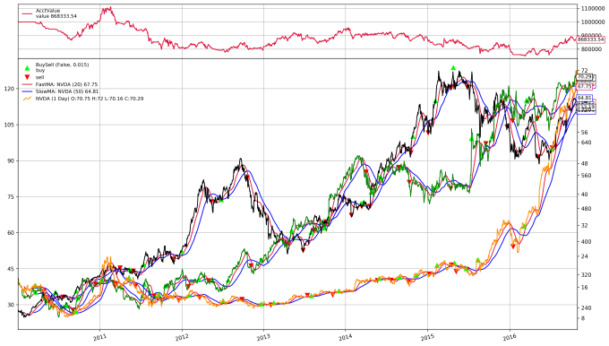
cerebro.plot(iplot=True, volume=False)
[[]]
cerebro.broker.getvalue()
822546.6400000001
This strategy is not doing well at all; it’s losing money by a hefty margin. Looking at this plot at the line for NVDA (the orange line; sadly, the legend generated here is not very good and I don’t know how to fix it, but I’m not worried about that issue right now), we see a lot of trading in a period that appears to be doldrums, driving up expenses.
Is there hope?
Optimization
We may attempt to optimize the window length parameters for the fast and slow moving averages and find a combination that is profitable in the backtest. Now, in the real world, traders need to be wary of overfitting. I’m not going to look at the overfitting problem right now; I’m just interested in how one may attempt to optimize using backtrader.
Here I judge strategies by the value of the final account at the end of the optimization period. The strategy that leads to the greatest profit will be the strategy I prefer. This is not the only criteria by which we may want to judge a strategy, and in the real world judging a strategy just by its end profitability may lead to disaster. Nevertheless, being a simple person, that is precisely how I will judge my strategies for now.
What I do is define a backtrader Analyzer. This is an object that computes statistics for strategies, like Sharpe ratios, maximum drawdown, etc. They often return a handful of quantities per asset traded or per account.
My analyzer, AcctStats, has an __init__() method that gets the starting account value (always \$1,000,000 in this case), a stop() method called after the last bar of the backtest has been processed that gets the final account value, and a get_analysis() method that returns a dict with these statistics, along with the account’s growth and return over the period. I define the analyzer below.
class AcctStats(bt.Analyzer):
    """A simple analyzer that gets the gain in the value of the account; should be self-explanatory"""

    def __init__(self):
        self.start_val = self.strategy.broker.get_value()
        self.end_val = None

    def stop(self):
        self.end_val = self.strategy.broker.get_value()

    def get_analysis(self):
        return {"start": self.start_val, "end": self.end_val,
                "growth": self.end_val - self.start_val, "return": self.end_val / self.start_val}
When optimizing, we need possible parameter values. In quantstrat, we would define parameter distributions, restrictions, and quantstrat would automatically pick either all possible legal combinations or a random sample of combinations of parameter values. backtrader, on the other hand, will expect a list of parameter values you wish to test, and will test every possible combination; it does not automatically randomize or impose parameter restrictions. I will need to do this myself. The code below generates possible parameter combinations. Notice the use of tuples. This explains my desire for an alternative parameter encoding in the strategy SMAC.
# Generate random combinations of fast and slow window lengths to test
windowset = set()    # Use a set to avoid duplicates
while len(windowset) < 40:
    f = random.randint(1, 10) * 5
    s = random.randint(1, 10) * 10
    if f > s:    # Cannot have the fast moving average have a longer window than the slow, so swap
        f, s = s, f
    elif f == s:    # Cannot be equal, so do nothing, discarding results
        pass
    windowset.add((f, s))

windows = list(windowset)
windows
[(15, 20),
 (5, 50),
 (45, 80),
 (10, 15),
 (20, 60),
 (30, 80),
 (40, 60),
 (35, 80),
 (40, 80),
 (20, 100),
 (5, 30),
 (10, 30),
 (25, 30),
 (10, 80),
 (20, 30),
 (35, 40),
 (45, 70),
 (35, 50),
 (20, 40),
 (35, 90),
 (25, 60),
 (40, 100),
 (10, 40),
 (10, 70),
 (10, 50),
 (15, 60),
 (35, 60),
 (10, 90),
 (15, 100),
 (20, 50),
 (5, 100),
 (10, 10),
 (10, 45),
 (25, 90),
 (5, 20),
 (40, 40),
 (15, 40),
 (30, 50),
 (10, 60),
 (30, 45)]
Now I create a new Cerebro object that will handle optimization. Supposedly, it is possible to parallelize this (computationally taxing) procedure, and backtrader attempts to do this automatically, but the computer I’m running from (a cheap one I bought for barely over \$200 that doesn’t even have 32 GB of hard-drive space) either can’t or shouldn’t attempt to take advantage of this. What’s worse, though, is that trying to allow parallelized operation throws errors (you can experiment by removing maxcpus=1 and running my code). I don’t know why they are occurring. It looks as if objects are not propagating across CPUs.
That issue aside, I optimize the strategy by using the Cerebro method optstrategy() instead of addstrategy() when adding the strategy, and passing the possible values of the parameters I want to optimize. Notice that the parameters optim and optim_fs in the method call are referring to parameters of the Strategy object; they are not arguments of the method. I pass the list of window parameters to test to the optim_fs parameter, along with the analyzer and sizer.
optorebro = bt.Cerebro(maxcpus=1)    # Object for optimization (setting maxcpus to 1
                                     # cuz parallelization throws errors; why?)
optorebro.broker.set_cash(1000000)
optorebro.broker.setcommission(0.02)
optorebro.optstrategy(SMAC, optim=True,    # Optimize the strategy (use optim variant of SMAC)...
                      optim_fs=windows)    # ... over all possible combinations of windows
for s in symbols:
    data = bt.feeds.YahooFinanceData(dataname=s, fromdate=start, todate=end)
    optorebro.adddata(data)

optorebro.addanalyzer(AcctStats)
optorebro.addsizer(PropSizer)
Then I optimize.
%time res = optorebro.run() # Perform the optimization
CPU times: user 13min 3s, sys: 4.61 s, total: 13min 7s
Wall time: 26min 12s
What’s returned is a list of objects that can be used to see the results of the optimization. In particular, I can see the parameters used for each round and get the analysis produced by the analyzer for each run. With the code below, I can organize this information into a pandas DataFrame.
# Store results of optimization in a DataFrame
return_opt = DataFrame({r[0].params.optim_fs: r[0].analyzers.acctstats.get_analysis() for r in res}
                      ).T.loc[:, ['end', 'growth', 'return']]
return_opt
| end | growth | return | ||
|---|---|---|---|---|
| 5 | 20 | 197486.24 | -802513.76 | 0.197486 |
| 30 | 334366.62 | -665633.38 | 0.334367 | |
| 50 | 518615.32 | -481384.68 | 0.518615 | |
| 100 | 871081.12 | -128918.88 | 0.871081 | |
| 10 | 10 | 1000000.00 | 0.00 | 1.000000 |
| 15 | 114558.28 | -885441.72 | 0.114558 | |
| 30 | 545751.16 | -454248.84 | 0.545751 | |
| 40 | 562529.38 | -437470.62 | 0.562529 | |
| 45 | 685313.28 | -314686.72 | 0.685313 | |
| 50 | 825899.84 | -174100.16 | 0.825900 | |
| 60 | 907465.20 | -92534.80 | 0.907465 | |
| 70 | 1078015.60 | 78015.60 | 1.078016 | |
| 80 | 1073558.70 | 73558.70 | 1.073559 | |
| 90 | 1063163.98 | 63163.98 | 1.063164 | |
| 15 | 20 | 237150.30 | -762849.70 | 0.237150 |
| 40 | 719085.78 | -280914.22 | 0.719086 | |
| 60 | 998381.28 | -1618.72 | 0.998381 | |
| 100 | 1163165.78 | 163165.78 | 1.163166 | |
| 20 | 30 | 565431.56 | -434568.44 | 0.565432 |
| 40 | 715309.22 | -284690.78 | 0.715309 | |
| 50 | 822546.64 | -177453.36 | 0.822547 | |
| 60 | 1004484.80 | 4484.80 | 1.004485 | |
| 100 | 1274192.36 | 274192.36 | 1.274192 | |
| 25 | 30 | 340475.46 | -659524.54 | 0.340475 |
| 60 | 1132969.20 | 132969.20 | 1.132969 | |
| 90 | 1156377.10 | 156377.10 | 1.156377 | |
| 30 | 45 | 788541.22 | -211458.78 | 0.788541 |
| 50 | 929846.52 | -70153.48 | 0.929847 | |
| 80 | 1274546.96 | 274546.96 | 1.274547 | |
| 35 | 40 | 471646.44 | -528353.56 | 0.471646 |
| 50 | 826959.20 | -173040.80 | 0.826959 | |
| 60 | 1047809.46 | 47809.46 | 1.047809 | |
| 80 | 1344409.94 | 344409.94 | 1.344410 | |
| 90 | 1178842.16 | 178842.16 | 1.178842 | |
| 40 | 40 | 1000000.00 | 0.00 | 1.000000 |
| 60 | 963963.06 | -36036.94 | 0.963963 | |
| 80 | 1302832.48 | 302832.48 | 1.302832 | |
| 100 | 1215086.58 | 215086.58 | 1.215087 | |
| 45 | 70 | 1034375.24 | 34375.24 | 1.034375 |
| 80 | 1175149.84 | 175149.84 | 1.175150 |
return_opt.sort_values("growth", ascending=False)
| end | growth | return | ||
|---|---|---|---|---|
| 35 | 80 | 1344409.94 | 344409.94 | 1.344410 |
| 40 | 80 | 1302832.48 | 302832.48 | 1.302832 |
| 30 | 80 | 1274546.96 | 274546.96 | 1.274547 |
| 20 | 100 | 1274192.36 | 274192.36 | 1.274192 |
| 40 | 100 | 1215086.58 | 215086.58 | 1.215087 |
| 35 | 90 | 1178842.16 | 178842.16 | 1.178842 |
| 45 | 80 | 1175149.84 | 175149.84 | 1.175150 |
| 15 | 100 | 1163165.78 | 163165.78 | 1.163166 |
| 25 | 90 | 1156377.10 | 156377.10 | 1.156377 |
| 60 | 1132969.20 | 132969.20 | 1.132969 | |
| 10 | 70 | 1078015.60 | 78015.60 | 1.078016 |
| 80 | 1073558.70 | 73558.70 | 1.073559 | |
| 90 | 1063163.98 | 63163.98 | 1.063164 | |
| 35 | 60 | 1047809.46 | 47809.46 | 1.047809 |
| 45 | 70 | 1034375.24 | 34375.24 | 1.034375 |
| 20 | 60 | 1004484.80 | 4484.80 | 1.004485 |
| 40 | 40 | 1000000.00 | 0.00 | 1.000000 |
| 10 | 10 | 1000000.00 | 0.00 | 1.000000 |
| 15 | 60 | 998381.28 | -1618.72 | 0.998381 |
| 40 | 60 | 963963.06 | -36036.94 | 0.963963 |
| 30 | 50 | 929846.52 | -70153.48 | 0.929847 |
| 10 | 60 | 907465.20 | -92534.80 | 0.907465 |
| 5 | 100 | 871081.12 | -128918.88 | 0.871081 |
| 35 | 50 | 826959.20 | -173040.80 | 0.826959 |
| 10 | 50 | 825899.84 | -174100.16 | 0.825900 |
| 20 | 50 | 822546.64 | -177453.36 | 0.822547 |
| 30 | 45 | 788541.22 | -211458.78 | 0.788541 |
| 15 | 40 | 719085.78 | -280914.22 | 0.719086 |
| 20 | 40 | 715309.22 | -284690.78 | 0.715309 |
| 10 | 45 | 685313.28 | -314686.72 | 0.685313 |
| 20 | 30 | 565431.56 | -434568.44 | 0.565432 |
| 10 | 40 | 562529.38 | -437470.62 | 0.562529 |
| 30 | 545751.16 | -454248.84 | 0.545751 | |
| 5 | 50 | 518615.32 | -481384.68 | 0.518615 |
| 35 | 40 | 471646.44 | -528353.56 | 0.471646 |
| 25 | 30 | 340475.46 | -659524.54 | 0.340475 |
| 5 | 30 | 334366.62 | -665633.38 | 0.334367 |
| 15 | 20 | 237150.30 | -762849.70 | 0.237150 |
| 5 | 20 | 197486.24 | -802513.76 | 0.197486 |
| 10 | 15 | 114558.28 | -885441.72 | 0.114558 |
It seems that the combination (35, 80) lead to the most profit, a strangely convenient combination. Let’s see the results of this combination in more detail, by running the earlier backtest but with a new Cerebro object containing the new parameter values suggested by the optimization.
fast_opt, slow_opt = return_opt.sort_values("growth", ascending=False).iloc[0].name

cerebro_opt = bt.Cerebro(stdstats=False)
cerebro_opt.broker.set_cash(1000000)
cerebro_opt.broker.setcommission(0.02)
cerebro_opt.addobserver(AcctValue)
cerebro_opt.addstrategy(SMAC, fast=fast_opt, slow=slow_opt)
cerebro_opt.addsizer(PropSizer)

cerebro_test = deepcopy(cerebro_opt)

is_first = True
plot_symbols = ["AAPL", "GOOG", "NVDA"]
#plot_symbols = []
for s in symbols:
    data = bt.feeds.YahooFinanceData(dataname=s, fromdate=start, todate=end)
    if s in plot_symbols:
        if is_first:
            data_main_plot = data
            is_first = False
        else:
            data.plotinfo.plotmaster = data_main_plot
    else:
        data.plotinfo.plot = False
    cerebro_opt.adddata(data)
%time cerebro_opt.run()
CPU times: user 18.3 s, sys: 112 ms, total: 18.4 s
Wall time: 40.7 s


[]
cerebro_opt.broker.get_value()
1344409.9400000002
cerebro_opt.plot(iplot=True, volume=False)
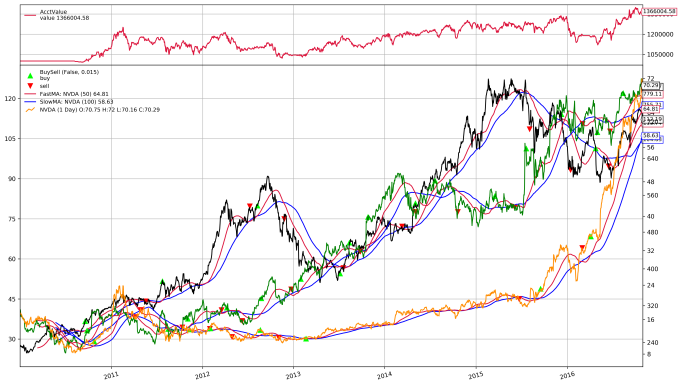
[[]]
It doesn’t look bad, but how do we know we didn’t overfit?
Let’s look at how this new parameter combination does out-of-sample. Notice that I’m using a copy of cerebro_opt created with the function deepcopy() (for copying Python objects), then feed the data for the symbols from a different time frame.
start_test = datetime.datetime(2016, 9, 1)
end_test = datetime.datetime(2017, 5, 31)
is_first = True
plot_symbols = ["AAPL", "GOOG", "NVDA"]
#plot_symbols = []
for s in symbols:
    data = bt.feeds.YahooFinanceData(dataname=s, fromdate=start_test, todate=end_test)
    if s in plot_symbols:
        if is_first:
            data_main_plot = data
            is_first = False
        else:
            data.plotinfo.plotmaster = data_main_plot
    else:
        data.plotinfo.plot = False
    cerebro_test.adddata(data)
%time cerebro_test.run()
CPU times: user 4.44 s, sys: 108 ms, total: 4.55 s
Wall time: 24.2 s


[]
cerebro_test.plot(iplot=True, volume=False)
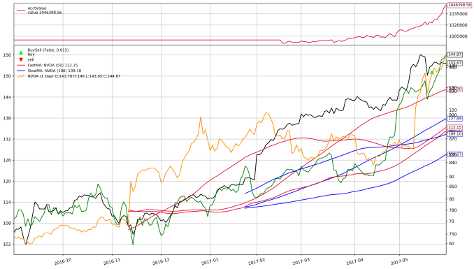
[[]]
cerebro_test.broker.get_value()
1122338.9
The out-of-sample result is actually not that bad. That said, I would not feel safe trading this strategy. Checking one out-of-sample instance is not enough to defend against overfitting. I would want to see a walk-forward analysis on top of a single out-of-sample check. I may discuss this topic more in a later article.
Conclusion
backtrader appears to be more complicated than quantstrat and takes more effort to get “up-and-running”. That is not necessarily a bad thing. backtrader looks much more flexible than quantstrat, and I am better able to predict what will happen when I use a backtrader Cerebro object as opposed to whatever quantstrat does.
When I use backtrader and read through its documentation I get the impression that its author uses backtrader and envisions backtrader being used in a non-interactive way, such as from a command line as a command line application. (Which isn’t wrong, per se; you can do a lot from the command line, especially on a Linux system). backtrader supports better plotting in a Jupyter notebook, but few other examples exist. That isn’t to say that backtrader cannot be used interactively (I wrote this article in a Jupyter notebook), but some features that work well in an interactive environment, such as pandas DataFrames, are not supported well. It seems that once a backtest is complete, accessing the data retrospectively isn’t easy, if possible. There is no pandas DataFrame containing trade data, or the value of the account, or other values that may have been tracked. However, one could load these into the environment for interactive use if they wrote a log file that could then be read in, such as a CSV file.
Since I envision strategy development taking place most naturally in an interactive setting, I think there should be better support for it. For example, I would like to be able to log to, say, a JSON string or Python dict or pandas DataFrame directly so I can work with that data right away. I hope this type of functionality is planned for the future. I can live saving output to separate files for now, though. Furthermore, usually when I want all values of, say, the account, I want them for a plot. If I want that data for a statistical analysis, I can use an analyzer.
Make no mistake, though: I like backtrader. In addition to liking its architecture, the package has stellar documentation and a great introductory tutorial. Its creator appears to be very active in his community, answering users questions promptly. He regularly keeps his own blog with not only news about the software but many useful tutorials addressing common tasks people struggle with. He’s done excellent work and I hope to see other users of backtrader in the community asking questions and contributing content. I’m hoping that someone from that community will read this article and offer advice for some of the issues I encountered. (If so, please comment.)
That said, considering I’ve been presenting backtrader in contrast to quantstrat and have been criticizing the latter a lot, I don’t want to imply that the developers of quantstrat are incompetent or lazy. That package clearly involved a lot of work and at one point I thought it could do no wrong. It’s also the only other backtesting platform I know. Bear in mind give criticisms directly, stating precisely what I do and do not like while attempting to be constructive and suggest improvement. I appreciate the developers’ work and I would like to revisit it in the future.
For now, though, I want to look more at backtrader. In particular, I want to employ a cross-validation scheme. I’ve badly wanted to do this type of analysis and can’t wait to try it finally.

Thanks for this post. Very helpful.
The comment fragment “always mens the” should read “always means the”.
LikeLike
Thank you for this post. It helped me understand the backtrader optimization process
LikeLike